Finding the Best Cherry Blossom Streets in Vancouver

Geospatial Analysis, Route Optimization, and Science Communication with R

Daniel Chen

2026-04-30

Motivation

Every spring Vancouver gets buried in cherry blossoms
The Vancouver Cherry Blossom Festival runs ~March 27 – April 17
But which streets are actually worth visiting?
And could you see the best of them in a single run?

The Goal

Find all Japanese flowering cherry trees in Vancouver
Identify the streets (and neighbourhoods) with the highest density
Build an optimized route to visit the top streets in one trip

All code: https://github.com/chendaniely/yvr-cherry-blossoms

The Full Pipeline

data/original/          ← Vancouver Open Data (raw GeoJSON)
    ↓ code/01-clean/
data/final/             ← cherry_blossoms.geojson, streets.geojson
    ↓ code/02-street_tree/
data/processed/         ← snapped-tree-street.geojson, streets_counted.geojson
    ↓ results/street_results/README.qmd
data/processed/         ← top30_streets.geojson
    ↓ results/tsp_route/README.qmd + code/03-routes/gpx_export.R
data/routes/            ← 4 GPX files

make data      # run all R cleaning + analysis scripts
make results   # render all Quarto result pages
make routes    # generate GPX files

Shout Out: Kyle Walker, PhD

The project that started it all:

Kyle Walker — great R packages for spatial work:

{tidycensus}, {tigris}, {crsuggest}
{mapgl} - every interactive map in this talk

Then I saw this post:

“New in the spopt-r #rstats package: route optimization. Solve the classic Traveling Salesman Problem for a single driver or optimize a fleet by solving the Vehicle Routing Problem.”

Find Kyle:

{spopt} - R route optimization:

Outline

Setup

GIS concepts review
Vancouver Open Data Portal
The tree & street data

Analysis

Building the initial map
Neighbourhood-level questions
Street-level density
Route optimization

GIS Concepts Review

Previous R-Ladies Talks

Create Custom Webpages with R and Quarto - Grace (March 2026)

R-Ladies YVR · Meetup event

Intro to Spatial Data in R - Véronique & Johannes (2025)

R-Ladies YVR · Meetup event

If you missed those talks - this section is a quick refresher on the GIS concepts we’ll use today.

What is GIS?

Geographic Information System - tools for capturing, storing, analyzing spatial data

Vector data (what we use today)

Points - individual trees 🌸
Lines - street segments 🛣️
Polygons - neighbourhoods 🗺️

Raster data (not today)

Grids of pixels
Satellite imagery, elevation
{terra}, {stars}

Coordinate Reference Systems

Every spatial dataset needs a CRS - defines how coordinates map to Earth’s surface

library(sf)

# WGS84 - latitude/longitude (degrees) - good for display
trees <- st_read("submodule/yvr-cherry-blossoms/data/original/public-trees.geojson")

Warning

Mix up your CRS and you’ll get wrong results with no error message.

Coordinate Reference Systems

Reading layer `public-trees' from data source 
  `/Users/dan/git/hub/rladies-2026-04-30-blossoms/submodule/yvr-cherry-blossoms/data/original/public-trees.geojson' 
  using driver `GeoJSON'
replacing null geometries with empty geometries
Simple feature collection with 186342 features and 11 fields (with 1 geometry empty)
Geometry type: POINT
Dimension:     XY
Bounding box:  xmin: -123.2367 ymin: 49.2002 xmax: -123.0233 ymax: 49.30998
Geodetic CRS:  WGS 84

st_crs(trees)  # EPSG:4326

Coordinate Reference System:
  User input: WGS 84 
  wkt:
GEOGCRS["WGS 84",
    DATUM["World Geodetic System 1984",
        ELLIPSOID["WGS 84",6378137,298.257223563,
            LENGTHUNIT["metre",1]]],
    PRIMEM["Greenwich",0,
        ANGLEUNIT["degree",0.0174532925199433]],
    CS[ellipsoidal,2],
        AXIS["geodetic latitude (Lat)",north,
            ORDER[1],
            ANGLEUNIT["degree",0.0174532925199433]],
        AXIS["geodetic longitude (Lon)",east,
            ORDER[2],
            ANGLEUNIT["degree",0.0174532925199433]],
    ID["EPSG",4326]]

# UTM Zone 10N - metres - good for distance calculations
trees_utm <- st_transform(trees, 32610)

CRS Alphanumeric Soup

EPSG:4326 = WGS84

EPSG - a registry of named coordinate systems (like a phone book for CRS)
4326 - the ID for WGS84 in that registry
WGS84 - the actual name: World Geodetic System 1984
What you get: lat/lon in degrees, used by GPS, Google Maps, GeoJSON

EPSG:32610 = UTM Zone 10N

32610 - EPSG ID for UTM Zone 10N (covers BC/Pacific Northwest)
UTM - Universal Transverse Mercator, a family of projected systems
Zone 10N - the specific slice of the globe (Vancouver falls here)
What you get: X/Y in metres - essential for distance calculations

Tip

Rule of thumb: use 4326 for display/storage, 32610 for anything involving distance or area in BC.

Key `{sf}` Operations We’ll Use

Function	What it does
`st_read()`	Load geojson / shapefile / etc
`st_transform()`	Reproject to a new CRS
`st_nearest_feature()`	Snap each point to closest line
`st_length()`	Length of line in CRS units
`st_join()`	Spatial join (like SQL JOIN but spatial)
`st_buffer()`	Buffer geometries by a distance
`st_union()`	Merge geometries together

Key R Packages

library(sf)          # spatial data I/O and operations
library(dplyr)       # data manipulation
library(mapgl)       # interactive maps (MapLibre GL)
library(sfnetworks)  # street/graph networks
library(igraph)      # graph algorithms (TSP cost matrix)
library(spopt)       # route optimization (TSP solver)
library(osmdata)     # OpenStreetMap data queries

Key R Packages

Vancouver Open Data Portal

opendata.vancouver.ca

https://opendata.vancouver.ca/pages/home/

The City of Vancouver publishes hundreds of datasets under open licenses:

Trees, parks, bike lanes, zoning, permits, 3D buildings…

We’ll use 5 datasets today:

Dataset	Format	What it contains
`public-trees`	GeoJSON	All ~150k city trees
`public-streets`	GeoJSON	City-maintained streets
`non-city-streets`	GeoJSON	Private/strata streets
`lanes`	GeoJSON	Lane segments
`local-area-boundary`	GeoJSON	22 neighbourhood polygons

Reading the Data

library(sf)

# All datasets are GeoJSON - sf reads them directly
trees        <- st_read("submodule/yvr-cherry-blossoms/data/original/public-trees.geojson")

glimpse(trees)

Reading the Data

Rows: 186,342
Columns: 12
$ asset_id      <int> 270046, 270058, 270059, 270079, 270081, 270085, 270090, …
$ address       <chr> "6110 ST. CLAIR PLACE", "3444 ST. CATHERINES ST", "3104 …
$ common_name   <chr> "CHERRY, PLUM OR PEACH SPECIES", "JAPANESE SNOWBELL", "W…
$ genus_name    <chr> "PRUNUS", "STYRAX", "TSUGA", "FRAXINUS", "PARROTIA", "FR…
$ species_name  <chr> "SPECIES", "JAPONICUS", "HETEROPHYLLA", "ORNUS", "PERSIC…
$ cultivar_name <chr> "NONE", "NONE", "NONE", "ARIE PETERS", "PERSIAN SPIRE", …
$ height_m      <dbl> 13.7, 4.6, 19.8, 4.6, 4.6, 5.0, 4.6, 4.6, 4.6, 4.6, 4.6,…
$ diameter_cm   <dbl> 88.9, 7.6, 66.0, 5.1, 7.6, 8.0, 7.6, 7.6, 7.6, 7.6, 7.6,…
$ date_planted  <date> NA, 2021-12-15, NA, 2023-03-09, 2021-03-25, 2022-12-16,…
$ geom          <chr> NA, NA, NA, NA, NA, NA, NA, NA, NA, NA, NA, NA, NA, NA, …
$ geo_point_2d  <chr> "{ \"lon\": -123.19037399947032, \"lat\": 49.23186499926…
$ geometry      <POINT [°]> POINT (-123.1904 49.23186), POINT (-123.0856 49.25…

# Rows: 150,016
# $ tree_id       <int>
# $ common_name   <chr>  "JAPANESE FLOWERING CHERRY", ...
# $ species_name  <chr>  "SERRULATA", ...
# $ cultivar_name <chr>  "ACCOLADE", ...
# $ date_planted  <date>
# $ height_m      <dbl>
# $ diameter_cm   <dbl>
# $ geometry      <POINT [°]>

Reading the Data

Reading layer `public-trees' from data source 
  `/Users/dan/git/hub/rladies-2026-04-30-blossoms/submodule/yvr-cherry-blossoms/data/original/public-trees.geojson' 
  using driver `GeoJSON'
replacing null geometries with empty geometries
Simple feature collection with 186342 features and 11 fields (with 1 geometry empty)
Geometry type: POINT
Dimension:     XY
Bounding box:  xmin: -123.2367 ymin: 49.2002 xmax: -123.0233 ymax: 49.30998
Geodetic CRS:  WGS 84

streets_city <- st_read("submodule/yvr-cherry-blossoms/data/original/public-streets.geojson")

Reading layer `public-streets' from data source 
  `/Users/dan/git/hub/rladies-2026-04-30-blossoms/submodule/yvr-cherry-blossoms/data/original/public-streets.geojson' 
  using driver `GeoJSON'
Simple feature collection with 17067 features and 3 fields
Geometry type: MULTILINESTRING
Dimension:     XY
Bounding box:  xmin: -123.2248 ymin: 49.20032 xmax: -123.0233 ymax: 49.2945
Geodetic CRS:  WGS 84

streets_priv <- st_read("submodule/yvr-cherry-blossoms/data/original/non-city-streets.geojson")

Reading layer `non-city-streets' from data source 
  `/Users/dan/git/hub/rladies-2026-04-30-blossoms/submodule/yvr-cherry-blossoms/data/original/non-city-streets.geojson' 
  using driver `GeoJSON'
Simple feature collection with 952 features and 4 fields
Geometry type: LINESTRING
Dimension:     XY
Bounding box:  xmin: -123.2299 ymin: 49.19895 xmax: -123.0124 ymax: 49.31404
Geodetic CRS:  WGS 84

lanes        <- st_read("submodule/yvr-cherry-blossoms/data/original/lanes.geojson")

Reading layer `lanes' from data source 
  `/Users/dan/git/hub/rladies-2026-04-30-blossoms/submodule/yvr-cherry-blossoms/data/original/lanes.geojson' 
  using driver `GeoJSON'
Simple feature collection with 7851 features and 3 fields
Geometry type: LINESTRING
Dimension:     XY
Bounding box:  xmin: -123.2223 ymin: 49.20096 xmax: -123.0233 ymax: 49.29374
Geodetic CRS:  WGS 84

neighbourhoods <- st_read("submodule/yvr-cherry-blossoms/data/original/local-area-boundary.geojson")

Reading layer `local-area-boundary' from data source 
  `/Users/dan/git/hub/rladies-2026-04-30-blossoms/submodule/yvr-cherry-blossoms/data/original/local-area-boundary.geojson' 
  using driver `GeoJSON'
Simple feature collection with 22 features and 2 fields
Geometry type: POLYGON
Dimension:     XY
Bounding box:  xmin: -123.2248 ymin: 49.19894 xmax: -123.0232 ymax: 49.29581
Geodetic CRS:  WGS 84

The Trees Data

Which Trees Are Cherry Blossoms?

150k+ trees in the dataset - most are not cherry blossoms.

Note

I had no idea there were so many different kinds of cherry blossom trees!

Strategy: filter common_name for trees that mention “cherry” AND (“japanese” OR “flower”)

library(stringr)

cherry_names <- unique(trees$common_name)[
  str_detect(unique(trees$common_name), "cherry|CHERRY")
]

jap_flower_cherry <- cherry_names[
  str_detect(cherry_names, "JAP|jap|FLOWER|flower")
]

jap_flower_cherry

Which Trees Are Cherry Blossoms?

 [1] "KWANZAN FLOWERING CHERRY"       "AKEBONO FLOWERING CHERRY"      
 [3] "SARGENT FLOWERING CHERRY"       "JAPANESE FLOWERING CHERRY"     
 [5] "UKON JAPANESE CHERRY"           "AMANOGAWA JAPANESE CHERRY"     
 [7] "WEEPING JAPANESE CHERRY"        NA                              
 [9] "OJOCHIN JAPANESE CHERRY"        "SHOGETSU JAPANESE CHERRY"      
[11] "DOUBLE WEEPING JAPANESE CHERRY"

Filtering the Trees

cherry_blossoms <- trees |>
  filter(common_name %in% jap_flower_cherry) |>
  mutate(
    age_years = as.numeric(
      difftime(Sys.Date(), as.Date(date_planted), units = "days")
    ) / 365.25
  )

nrow(cherry_blossoms)  # ~3,500 trees

10 species found:

JAPANESE FLOWERING CHERRY
AKEBONO FLOWERING CHERRY
KWANZAN FLOWERING CHERRY
… and more

Filtering the Trees

[1] 14992

Data Quality: A Frustration

Mature trees are more reliable bloomers. Filter by age?

# How complete is date_planted?
cherry_blossoms |>
  summarise(
    n           = n(),
    has_date    = sum(!is.na(date_planted)),
    pct_missing = mean(is.na(date_planted)) * 100
  )

  n     has_date  pct_missing
  3521  979       72.2

Warning

72% of trees have no planting date - age filtering is off the table.

Data Quality: A Frustration

Simple feature collection with 1 feature and 3 fields
Geometry type: MULTIPOINT
Dimension:     XY
Bounding box:  xmin: -123.2319 ymin: 49.20477 xmax: -123.0236 ymax: 49.30261
Geodetic CRS:  WGS 84
      n has_date pct_missing                       geometry
1 14992     4113    72.56537 MULTIPOINT ((-123.0256 49.2...

Falling Back to Size Proxies

Height and diameter are fully recorded - use them as size stand-ins:

# 100% complete
cherry_blossoms |>
  summarise(
    pct_height   = mean(!is.na(height_m))   * 100,  # 100%
    pct_diameter = mean(!is.na(diameter_cm)) * 100   # 100%
  )

# Thresholds (based on domain knowledge of Japanese flowering cherries)
min_height_m   <- 2.5   # metres
min_diameter_cm <- 7    # cm trunk diameter

# NOTE: in the final analysis, even filtering by these thresholds
# changes the result very little - most trees pass. We keep all trees.
blooming_trees <- cherry_blossoms

Falling Back to Size Proxies

Simple feature collection with 1 feature and 2 fields
Geometry type: MULTIPOINT
Dimension:     XY
Bounding box:  xmin: -123.2319 ymin: 49.20477 xmax: -123.0236 ymax: 49.30261
Geodetic CRS:  WGS 84
  pct_height pct_diameter                       geometry
1        100          100 MULTIPOINT ((-123.0256 49.2...

The Street Data

Three sources - combine them into one dataset:

streets_pub <- st_read(
  "submodule/yvr-cherry-blossoms/data/original/public-streets.geojson",
  quiet = TRUE
) |> st_transform(4326) |>
  mutate(street_type = "Public", street_label = hblock)

streets_non <- st_read(
  "submodule/yvr-cherry-blossoms/data/original/non-city-streets.geojson",
  quiet = TRUE
) |> st_transform(4326) |>
  mutate(
    street_type = "Non-city",
    street_label = if_else(
      !is.na(from_hblk) & from_hblk != "",
      paste(from_hblk, streetname), streetname
    )
  )

streets_lan <- st_read(
  "submodule/yvr-cherry-blossoms/data/original/lanes.geojson",
  quiet = TRUE
) |> st_transform(4326) |>
  mutate(street_type = "Lane",
         street_label = paste(from_hundred_block, std_street))

streets <- bind_rows(streets_pub, streets_non, streets_lan)
nrow(streets)

Note: each street is stored as individual block-level segments

The Street Data

[1] 25870

Building the Initial Map

First Map: Where Are the Trees?

Start simple - plot all cherry blossom trees with {mapgl}

library(mapgl)

maplibre(
  style = openfreemap_style("bright"),
  bounds = neighbourhoods
) |>
  add_circle_layer(
    id     = "trees",
    source = cherry_blossoms,
    circle_radius  = 3,
    circle_color   = "#e879a0",
    circle_opacity = 0.6
  )

First Map: Where Are the Trees?

Adding Neighbourhood Boundaries

maplibre(
  style = openfreemap_style("bright"),
  bounds = neighbourhoods
) |>
  add_line_layer(
    id         = "neighbourhood-borders",
    source     = neighbourhoods,
    line_color = "#d97706",
    line_width = 1.5,
    line_opacity = 0.8
  ) |>
  add_circle_layer(
    id     = "trees",
    source = cherry_blossoms,
    circle_radius  = 3,
    circle_color   = "#e879a0",
    circle_opacity = 0.6
  )

Adding Neighbourhood Boundaries

All Cherry Blossoms by Species

tree_variety_names <- sort(unique(cherry_blossoms$common_name))
tree_variety_colors <- colorRampPalette(
  c("#e879a0", "#a855f7", "#3b82f6", "#10b981", "#f59e0b")
)(length(tree_variety_names))

maplibre(
  style  = openfreemap_style("bright"),
  bounds = cherry_blossoms
) |>
  add_circle_layer(
    id     = "trees",
    source = cherry_blossoms,
    circle_color = match_expr(
      column = "common_name",
      values = tree_variety_names,
      stops  = tree_variety_colors
    ),
    circle_opacity = 0.7,
    tooltip = concat("<b>", get_column("common_name"), "</b>")
  ) |>
  add_categorical_legend(
    legend_title = "Tree variety",
    values       = tree_variety_names,
    colors       = tree_variety_colors,
    patch_shape  = "circle"
  )

All Cherry Blossoms by Species

Asking Questions

Which Neighbourhood Has Most?

We need to spatially join trees to neighbourhoods, then count:

tree_counts <- st_join(
  cherry_blossoms,
  neighbourhoods |> select(neighbourhood = name),
  join = st_within   # tree must fall INSIDE neighbourhood polygon
) |>
  st_drop_geometry() |>
  count(neighbourhood, name = "tree_count")

neighbourhoods <- neighbourhoods |>
  left_join(tree_counts, by = c("name" = "neighbourhood")) |>
  mutate(tree_count = replace_na(tree_count, 0))

Which Neighbourhood Has Most?

Raw Count vs Density

Raw count favours large neighbourhoods. Normalize by area:

neighbourhoods <- neighbourhoods |>
  mutate(
    area_km2     = as.numeric(st_area(geometry)) / 1e6,
    trees_per_km2 = tree_count / area_km2
  )

Top by raw count

Kitsilano, Hastings-Sunrise, Sunset…

Top by density

Mount Pleasant (!)

Raw Count vs Density

The Neighbourhood Choropleth

maplibre(style = openfreemap_style("bright"), bounds = neighbourhoods) |>
  add_fill_layer(
    id     = "neighbourhood-density",
    source = neighbourhoods,
    fill_color = interpolate(
      column = "trees_per_km2",
      values = c(0, median(neighbourhoods$trees_per_km2),
                    max(neighbourhoods$trees_per_km2)),
      stops  = c("#f7fcf0", "#41ab5d", "#00441b")
    ),
    fill_opacity = 0.75,
    tooltip = "tooltip_text"
  )

The Neighbourhood Choropleth

Surprising Finding #1

Mount Pleasant = highest density neighbourhood

David Lam Park (Downtown) = where the Festival is held

Why the paradox?

Downtown is geographically massive
Trees are concentrated in one small park
Density = trees ÷ area → big area = low density
But Mount Pleasant has trees spread across many residential streets

Which Streets Are Best?

Neighbourhoods give the overview - the actual experience is at street level.

Where do I take my mom?

Where can folks take photos?

Where are the hidden local gems?

Assign each tree to its nearest street segment
Count trees per segment
Normalize by length → trees per 100m
Rank and map

Street-Level Analysis

Example: Snapping - Toy Setup

Build a mini version with 4 streets and 9 trees:

street_colors <- c(
  "Oak St"     = "#e76f51",
  "Elm Ave"    = "#2a9d8f",
  "Cedar Rd"   = "#457b9d",
  "Maple Blvd" = "#9b5de5"
)

streets_toy <- st_sf(
  id   = 1:4,
  name = c("Oak St", "Elm Ave", "Cedar Rd", "Maple Blvd"),
  geometry = st_sfc(
    st_linestring(rbind(c(0, 0),  c(10, 0))),   # horizontal
    st_linestring(rbind(c(0, 8),  c(10, 8))),   # horizontal (upper)
    st_linestring(rbind(c(5, -1), c(5, 10))),   # vertical
    st_linestring(rbind(c(0, 5),  c(4, 10))),   # diagonal
    crs = 4326
  )
)

trees_toy <- st_sf(
  id = 1:9,
  geometry = st_sfc(
    st_point(c(1, -1.2)), st_point(c(3, 1.0)), st_point(c(7, -0.8)),
    st_point(c(2, 4.0)),  st_point(c(8, 4.5)), st_point(c(3, 7.0)),
    st_point(c(6, 9.2)),  st_point(c(9, 6.5)), st_point(c(4.5, 3.5)),
    crs = 4326
  )
)

Example: Snapping - Toy Setup

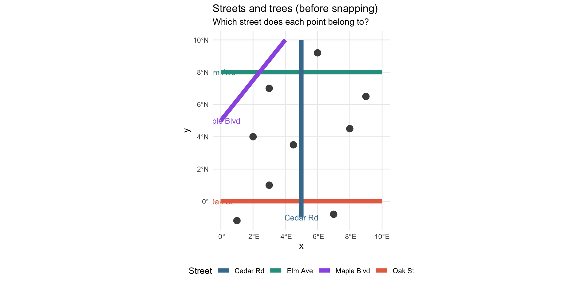
Example: Before Snapping

ggplot() +
  geom_sf(data = streets_toy, aes(color = name), linewidth = 2.5) +
  geom_sf_text(
    data = streets_toy,
    aes(label = name, color = name),
    size = 3.5, show.legend = FALSE
  ) +
  geom_sf(data = trees_toy, size = 4, shape = 16, color = "grey30") +
  scale_color_manual(values = street_colors, name = "Street") +
  labs(
    title    = "Streets and trees (before snapping)",
    subtitle = "Which street does each point belong to?"
  ) +
  theme_minimal() +
  theme(legend.position = "bottom")

Example: Before Snapping

Example: The Snap Operation

# One call assigns every tree to its nearest street
nearest_idx <- st_nearest_feature(trees_toy, streets_toy)

trees_toy <- trees_toy |>
  mutate(
    nearest_street_id   = nearest_idx,
    nearest_street_name = streets_toy$name[nearest_idx]
  )

tree_counts_toy <- trees_toy |>
  st_drop_geometry() |>
  count(nearest_street_id, nearest_street_name, name = "tree_count")

print(tree_counts_toy)

Example: The Snap Operation

  nearest_street_id nearest_street_name tree_count
1                 1              Oak St          3
2                 2             Elm Ave          2
3                 3            Cedar Rd          3
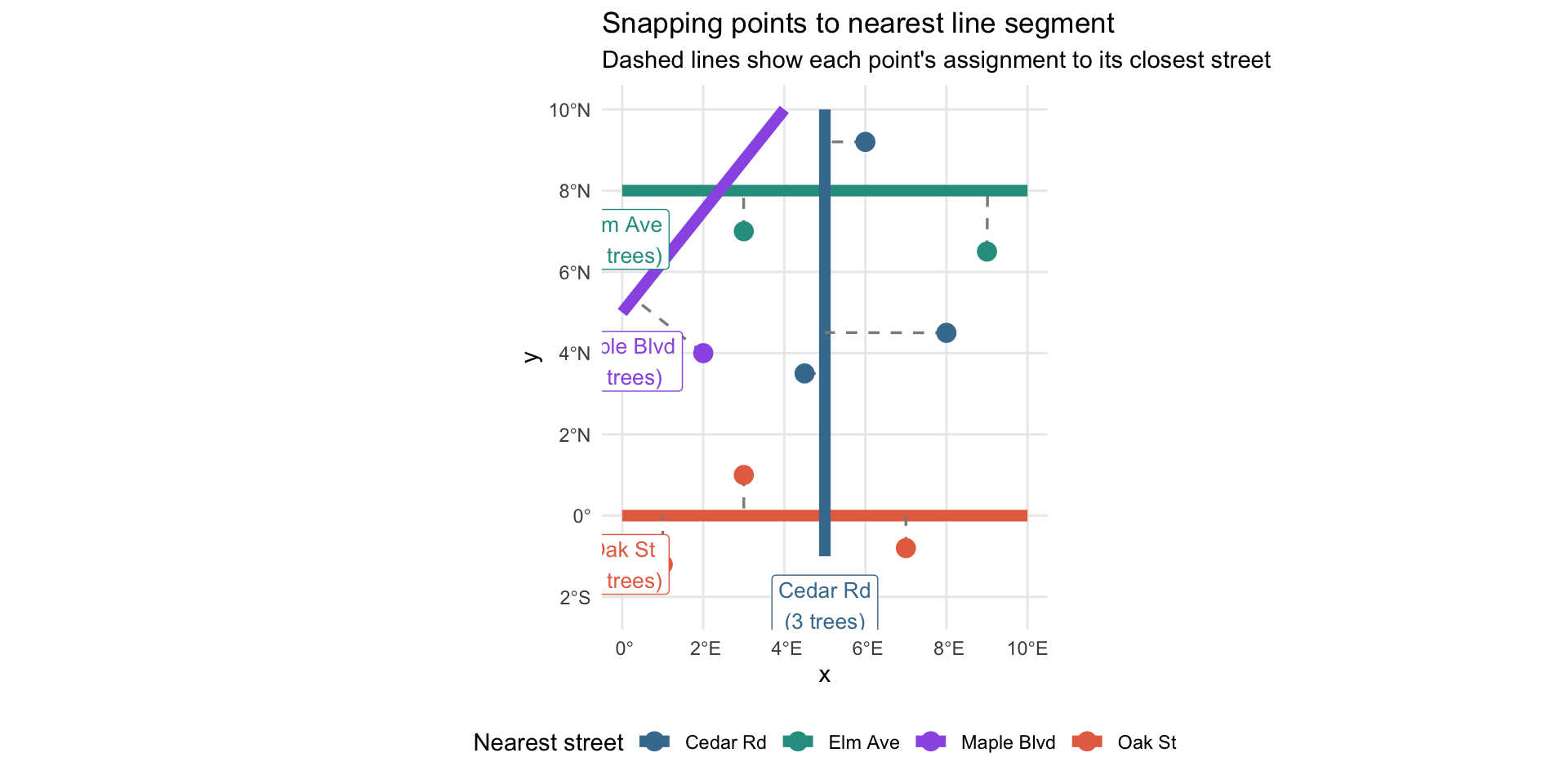
4                 4          Maple Blvd          1

Example: After Snapping

snap_lines <- trees_toy |>
  mutate(
    geometry = st_sfc(
      map2(
        geometry,
        streets_toy$geometry[nearest_street_id],
        ~ st_nearest_points(st_sfc(.x, crs = 4326), st_sfc(.y, crs = 4326))[[1]]
      ),
      crs = 4326
    )
  )

ggplot() +
  geom_sf(data = streets_toy, aes(color = name), linewidth = 2.5) +
  geom_sf(data = snap_lines, color = "grey55", linetype = "dashed", linewidth = 0.6) +
  geom_sf(data = trees_toy, aes(color = nearest_street_name), size = 4, shape = 16) +
  geom_sf_label(
    data = left_join(streets_toy, tree_counts_toy, by = c("id" = "nearest_street_id")),
    aes(label = paste0(name, "\n(", tree_count, " trees)"), color = name),
    size = 3.5, nudge_y = -1.2, show.legend = FALSE
  ) +
  scale_color_manual(values = street_colors, name = "Nearest street") +
  labs(
    title    = "Snapping points to nearest line segment",
    subtitle = "Dashed lines show each point's assignment to its closest street"
  ) +
  theme_minimal() +
  theme(legend.position = "bottom")

Example: After Snapping

Snapping Trees to Streets

st_nearest_feature() returns the index of the nearest feature - one call for all 3,500 trees:

# One function call assigns every tree to its nearest street
nearest_idx <- st_nearest_feature(cherry_blossoms, streets)

snapped <- cherry_blossoms |>
  mutate(
    street_id    = nearest_idx,
    street_label = streets$street_label[nearest_idx],
    street_type  = streets$street_type[nearest_idx]
  )

Note

Uses a spatial index under the hood - 3,500 trees × 50,000+ segments runs in seconds.

Snapping Trees to Streets

Counting Trees per Segment

tree_counts <- snapped |>
  st_drop_geometry() |>
  count(street_id, street_label, street_type,
        name = "tree_count")

streets_joined <- streets |>
  mutate(street_id = row_number()) |>
  left_join(tree_counts, by = "street_id")

# drop duplicate .y columns, rename .x → clean names, then compute length/density
streets_counted <- streets_joined |>
  select(-street_label.y, -street_type.y) |>
  rename(street_label = street_label.x, street_type = street_type.x) |>
  mutate(
    tree_count = replace_na(tree_count, 0),
    length_m   = as.numeric(st_length(geometry)),
    density    = tree_count / length_m * 100   # trees per 100m
  )

Counting Trees per Segment

Data Integrity Check

After the join, verify labels are consistent across segments:

label_mismatches <- streets_joined |>
  st_drop_geometry() |>
  filter(!is.na(street_label.y)) |>
  filter(street_label.x != street_label.y)

if (nrow(label_mismatches) > 0) {
  warning(sprintf(
    "%d segment(s) have mismatched labels - re-run clean scripts",
    nrow(label_mismatches)
  ))
} else {
  message("street_label check passed ✓")
}

Tip

Always validate spatial joins - silent mismatches are common.

Data Integrity Check

Example: Block-Level Segments

One “street” in the data is many separate block segments - pick one to see:

one_street <- streets |>
  filter(std_street == "GRANVILLE ST") |>
  mutate(
    segment_id    = row_number(),
    segment_color = rep(
      c("#e76f51", "#2a9d8f", "#457b9d", "#9b5de5"),
      length.out = n()
    )
  )

cat("Granville St has", nrow(one_street), "separate segments\n")

Note

Each colour is a separate row in the data - that’s why we need to aggregate before ranking streets.

Example: Block-Level Segments

Granville St has 82 separate segments

maplibre(bounds = one_street) |>
  add_line_layer(
    id     = "segments",
    source = one_street,
    line_color = get_column("segment_color"),
    line_width = 5,
    tooltip = concat(
      "Segment ", get_column("segment_id"), ": ", get_column("street_label")
    )
  )

Aggregating to Street Level

Each street has multiple block segments. Union them to see the whole street:

# summary table (no geometry - used for ranking)
street_summary <- streets_counted |>
  st_drop_geometry() |>
  filter(tree_count > 0) |>
  group_by(street_label, street_type) |>
  summarise(
    total_trees  = sum(tree_count),
    total_length = sum(length_m),
    n_segments   = n(),
    .groups = "drop"
  ) |>
  mutate(density = total_trees / total_length * 100)

# spatial version (geometry needed for mapping)
streets_sf <- streets_counted |>
  filter(tree_count > 0) |>
  group_by(street_label, street_type) |>
  summarise(
    total_trees  = sum(tree_count),
    total_length = sum(length_m),
    density      = sum(tree_count) / sum(length_m) * 100,
    geometry     = st_union(geometry),
    .groups = "drop"
  )

Aggregating to Street Level

Top Streets

# Top by raw count
top_by_count <- street_summary |>
  slice_max(total_trees, n = 20)

# Top by density - require ≥5 trees to suppress short stubs
# (a single tree on a 5m dead-end = 2000 trees/100m, meaningless)
top_by_density <- street_summary |>
  filter(total_trees >= 5) |>
  slice_max(density, n = 30)

Important

Without total_trees >= 5, a single tree on a 5m dead-end alley tops the rankings at 2,000 trees/100m.

Top Streets

The Top 30 Streets Map

maplibre(style = openfreemap_style("bright"), bounds = top30_stops) |>
  add_line_layer(
    id     = "streets-density",
    source = streets_dense,
    line_color = interpolate(
      column = "density",
      values = c(0, median(streets_dense$density),
                    max(streets_dense$density)),
      stops  = c("#edf8e9", "#74c476", "#00441b")
    ),
    line_width = interpolate(
      column = "density",
      values = c(0, max(streets_dense$density)),
      stops  = c(1.5, 6)
    ),
    popup = concat(
      "<b>", get_column("street_label"), "</b><br/>",
      "Trees / 100m: ", number_format(get_column("density"), 1)
    )
  )

The Top 30 Streets Map

Surprising Finding #2

Mount Pleasant has the highest neighbourhood density

but none of the top 30 densest streets

Why? Mount Pleasant trees are spread across many streets - great for wandering, but no single street is exceptionally dense.

The top streets cluster in West End / Yaletown, Kerrisdale, and East Vancouver.

The Top 10 Streets

#	Street	Trees / 100m	Total Trees
1	1400 HOMER ST	27.5	53
2	100 DRAKE ST	22.0	25
3	600 GILFORD ST	22.4	13
4	600 CHILCO ST	24.6	16
5	4500 BALACLAVA ST	22.7	12
6	2400 W 41ST AV	24.4	25
7	400 W 33RD AV	20.5	18
8	200 W 37TH AV	21.6	21
9	800 SALSBURY DRIVE	22.0	11
10	3100 RUPERT ST	19.3	18

Route Optimization

Travelling Salesperson Problem

Given N stops, find the shortest route visiting each exactly once.

NP-hard exactly - heuristics for anything practical
{spopt} by Kyle Walker: nearest-neighbour seed + 2-opt/or-opt improvement
Key input: a cost matrix of distances or travel times between every pair of stops

10 stops → 10! / 2 = 1,814,400 possible routes

Running the TSP

coords <- st_coordinates(top10_stops)
cost_matrix <- as.matrix(dist(coords))  # Euclidean - fast, good for prototyping

result <- route_tsp(
  top10_stops,
  start       = 1,     # Homer St (#1 ranked)
  end         = NULL,  # open route - no return to start
  cost_matrix = cost_matrix
)

meta <- attr(result, "spopt")
cat(sprintf("Improvement over nearest-neighbour: %.1f%%\n", meta$improvement_pct))

Running the TSP

Improvement over nearest-neighbour: 16.8%

stops_ordered <- result |>
  filter(!is.na(.visit_order)) |>
  arrange(.visit_order)
stops_ordered |> select(street_label, .visit_order)

Simple feature collection with 10 features and 2 fields
Geometry type: POINT
Dimension:     XY
Bounding box:  xmin: -123.1757 ymin: 49.23468 xmax: -123.0338 ymax: 49.2943
Geodetic CRS:  WGS 84
         street_label .visit_order                   geometry
1       1400 HOMER ST            1 POINT (-123.1262 49.27227)
2        100 DRAKE ST            2 POINT (-123.1231 49.27308)
3      600 GILFORD ST            3   POINT (-123.135 49.2938)
4       600 CHILCO ST            4   POINT (-123.137 49.2943)
5   4500 BALACLAVA ST            5 POINT (-123.1757 49.24542)
6      2400 W 41ST AV            6  POINT (-123.162 49.23468)
7       400 W 33RD AV            7 POINT (-123.1163 49.24101)
8       200 W 37TH AV            8 POINT (-123.1112 49.23711)
9  800 SALSBURY DRIVE            9 POINT (-123.0684 49.27731)
10     3100 RUPERT ST           10 POINT (-123.0338 49.25599)

Routing Geometry Was Off

route_tsp() returns the stop order - not the road paths between stops.

Drawing the actual route requires geometry connecting each stop in sequence.

What I tried

Build a road network from Vancouver street segments + sfnetworks, compute shortest paths, connect the dots

What happened

Routes didn’t follow roads - lines cut through blocks, missed turns, looked wrong

Why? Street Data ≠ Routing Data

Vancouver open data: block-level records - built for spatial joins, not routing
Tried full OpenStreetMap data - still had issues
Gaps in network topology, or geometry too messy for a DIY routing engine

The lesson: routing is a solved problem. Don’t rebuild it from scratch.

OSRM to the Rescue

TSP gives the order - OSRM gives actual road geometry:

library(httr)

osrm_route <- function(stops_sf, profile = "foot") {
  coords <- st_coordinates(stops_sf)
  coord_str <- paste(
    sprintf("%.6f,%.6f", coords[, 1], coords[, 2]),
    collapse = ";"
  )
  url <- sprintf(
    "https://router.project-osrm.org/route/v1/%s/%s?overview=full&geometries=geojson",
    profile, coord_str
  )
  content(GET(url))$routes[[1]]
}

Profiles: "foot" (sidewalks + paths) · "bike" (cycle lanes preferred)

OSRM to the Rescue

GPX Export

Make the route portable - Garmin, Strava, Komoot, AllTrails:

library(xml2)

write_gpx <- function(stops_sf, track_coords, name, path) {
  doc <- xml_new_root("gpx", version = "1.1",
    creator = "yvr-cherry-blossoms",
    xmlns   = "http://www.topografix.com/GPX/1/1")

  pts <- st_coordinates(stops_sf)
  for (i in seq_len(nrow(stops_sf))) {
    wpt <- xml_add_child(doc, "wpt",
      lat = sprintf("%.6f", pts[i, 2]),
      lon = sprintf("%.6f", pts[i, 1]))
    xml_add_child(wpt, "name",
      sprintf("Stop %d - %s", i, stops_sf$street_label[i]))
  }
  # ... track points from OSRM geometry added here
  write_xml(doc, path)
}

GPX Export

Cherry Blossom Marathon Route

Top 10 stops · 23.4 km (14.5 miles) straight-line · ~35 km road-following

Top 10 cherry blossom marathon route

For Cyclists: The Grand Tour

Top 30 stops · 34.7 km (21.6 miles) straight-line

Google Maps limits routes to 10 stops - split into 3 legs:

bike_stops <- tsp_result_30 |>
  filter(!is.na(.visit_order)) |>
  arrange(.visit_order) |>
  mutate(leg = ceiling(row_number() / 10))  # legs 1, 2, 3

# Generate Google Maps URL per leg
google_maps_url <- function(stops_sf) {
  stops_sf$google_address |>            # "HOMER ST, Vancouver, BC"
    URLencode(reserved = TRUE) |>
    paste(collapse = "/") |>
    paste0("https://www.google.com/maps/dir/", x = _)
}

urls <- lapply(1:3, \(i) google_maps_url(filter(bike_stops, leg == i)))
urls[[1]]

For Cyclists: The Grand Tour

[1] "https://www.google.com/maps/dir/1400%20HOMER%20ST%2C%20Vancouver%2C%20BC/100%20DRAKE%20ST%2C%20Vancouver%2C%20BC/600%20CHILCO%20ST%2C%20Vancouver%2C%20BC/600%20GILFORD%20ST%2C%20Vancouver%2C%20BC/1000%20MELVILLE%20ST%2C%20Vancouver%2C%20BC/800%20SALSBURY%20DRIVE%2C%20Vancouver%2C%20BC/2500%20OXFORD%20ST%2C%20Vancouver%2C%20BC/3000%20E%202ND%20AV%2C%20Vancouver%2C%20BC/3000%20E%207TH%20AV%2C%20Vancouver%2C%20BC/2600%20E%2022ND%20AV%2C%20Vancouver%2C%20BC"

Reflections

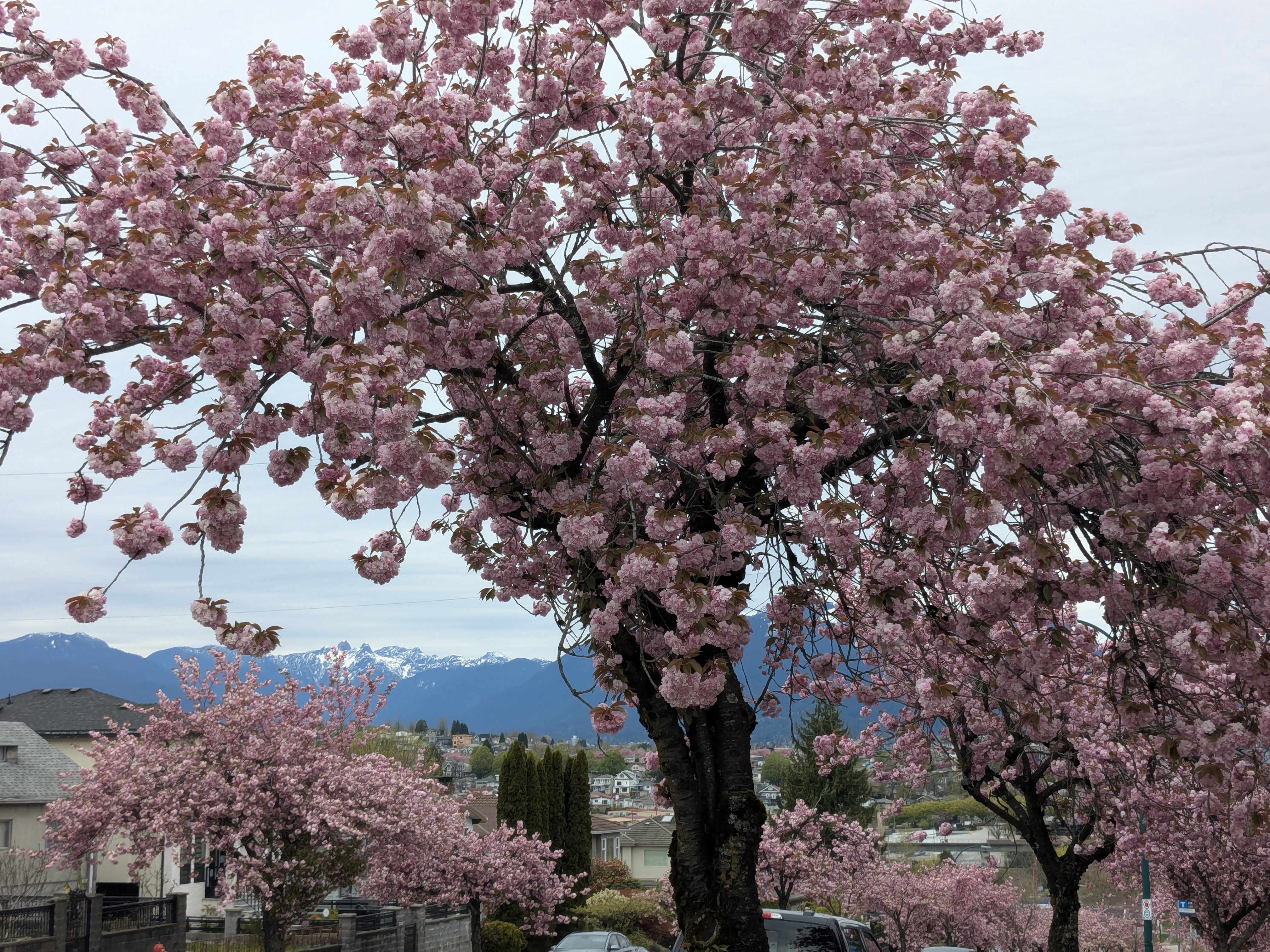
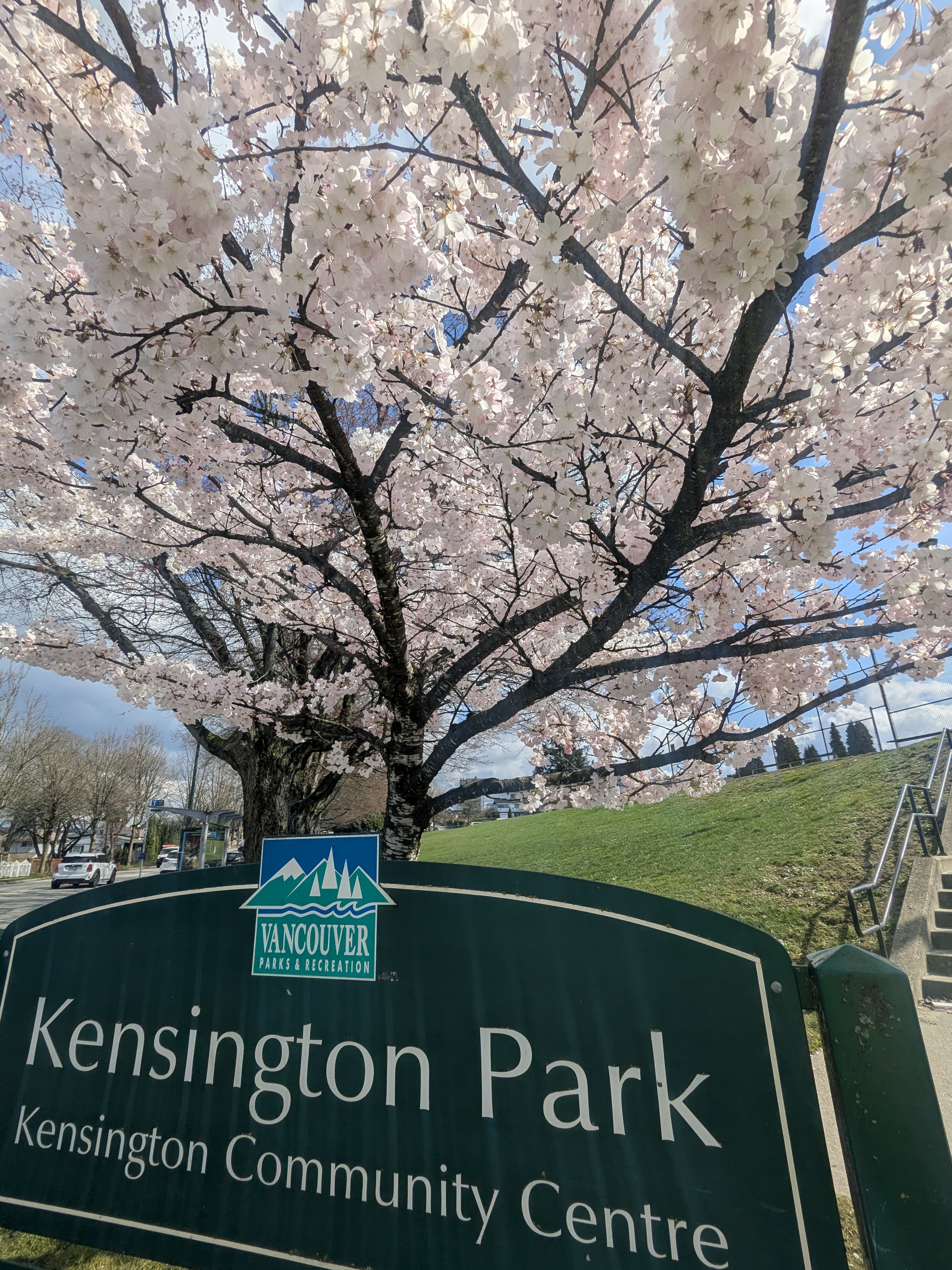
I Actually Ran It

Still in Bud: March 30th

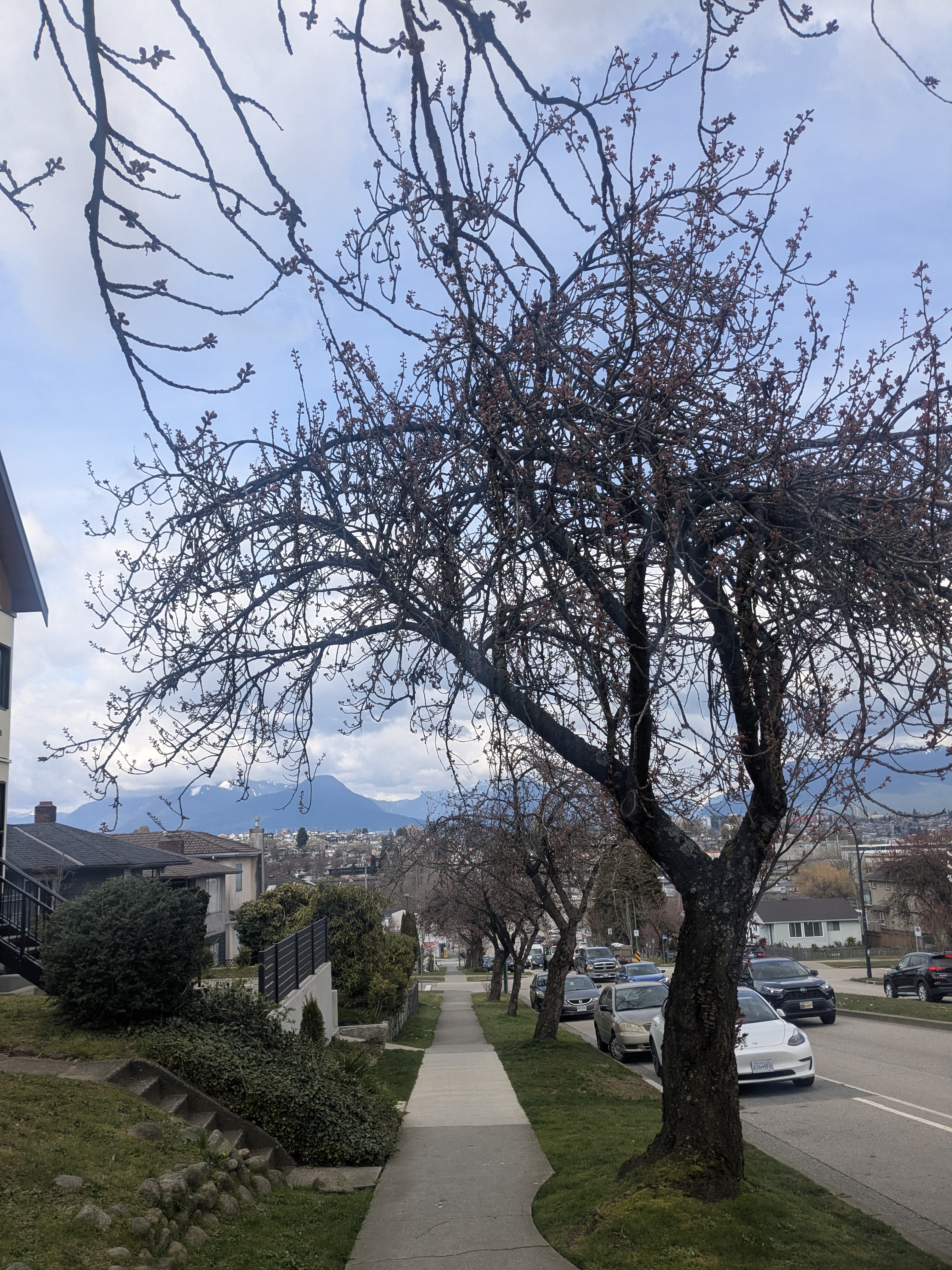
Peak Bloom: April 18th

Rupert St - with my mom, three weeks later:

Results & Reflection

What We Did

5 open Vancouver datasets → ~3,500 Japanese flowering cherry trees
Snapped trees to 50k street segments → density per 100m
Interactive maps: neighbourhood choropleth + top 30 streets
TSP: 10-stop running route and 30-stop cycling tour
GPX files ready to load into Strava / Garmin

Things Worth Remembering

st_nearest_feature() - point-to-line assignment in one call
Density without a minimum count is just noise from tiny alleys
Neighbourhood and street analysis ask different questions - both matter
TSP needs a cost matrix - Euclidean is fast, road network is honest
Clean the network (to_spatial_subdivision + to_spatial_smooth) before routing
OSRM turns stop order into actual road geometry

Where Claude Code Helped

Claude Code helped throughout:

Map aesthetics - described what I wanted, it wrote the {mapgl} layers
Google Maps URLs - split 30-stop tour into 3 legs of 10; shareable links
OSRM fallback - street data had geometry issues; Claude found OSRM as an alternative
Code comments - “why” not just “what”
Porting analysis to slides - scripts → slide-friendly code chunks
These slides - structure, submodule wiring, Kyle Walker shout-out
ASCII diagrams - mock up flow and structure diagrams
- Can also use Quarto + Mermaid diagrams

The code is not the hard part

AI can write the code. What it cannot do: ask the right question, recognize a wrong result, or know which assumption to challenge next. That is the skill worth building.

Open Data is Amazing

Vancouver Open Data Portal - free, well-documented, kept up to date:

Tree locations and dimensions
Street network (block-level segments)
Neighbourhood boundaries
Hundreds more datasets

Sharing Results with Quarto

Same R code → blog post via Quarto + GitHub Pages

Interactive maps embedded directly
GPX download links
No R required to read it
Analysis repo, talk, and blog are all Quarto documents

The Quarto stack

analysis.R
  ↓
results/README.qmd   ← blog post source
  ↓ quarto render
docs/index.html      ← GitHub Pages

Grace’s talk from last month covers exactly this.

Appreciating City Planners

The city has been deliberate about where these trees go:

Spread across many neighbourhoods, not concentrated in one spot
Different species bloom at different times → longer season overall
Even a single tree at an intersection makes a difference

Single cherry blossom tree — A single cherry blossom behind the Kensington Park Community Center sign

Next: Bloom-Aware Routes

The problem: routes show where trees are planted, not where they’re blooming

Confirmed on my March 30th run.

The idea

Crowd-sourced bloom photos: Facebook, Reddit, vcbf.ca
Estimate bloom timing per species
Species matters as much as microclimate
Build routes for trees actually blooming on a given day

What this becomes

Pick a date → route of currently-blooming streets:

Early March → early-blooming species
Peak season → full grand tour
Late April → late-blooming varieties only

The Blossoms Don’t Last Long

This season is over!

Resources

Analysis code: github.com/chendaniely/yvr-cherry-blossoms
Blog post: chendaniely.github.io
GPX files in the repo data/routes/

Finding the Best Cherry Blossom Streets in Vancouver

Motivation

The Goal

The Full Pipeline

Shout Out: Kyle Walker, PhD

Outline

GIS Concepts Review

Previous R-Ladies Talks

What is GIS?

Coordinate Reference Systems

Coordinate Reference Systems

CRS Alphanumeric Soup

Key {sf} Operations We’ll Use

Key R Packages

Key R Packages

Vancouver Open Data Portal

opendata.vancouver.ca

Reading the Data

Reading the Data

Reading the Data

The Trees Data

Which Trees Are Cherry Blossoms?

Which Trees Are Cherry Blossoms?

Filtering the Trees

Filtering the Trees

Data Quality: A Frustration

Data Quality: A Frustration

Falling Back to Size Proxies

Falling Back to Size Proxies

Falling Back to Size Proxies

The Street Data

The Street Data

Building the Initial Map

First Map: Where Are the Trees?

First Map: Where Are the Trees?

Adding Neighbourhood Boundaries

Adding Neighbourhood Boundaries

All Cherry Blossoms by Species

All Cherry Blossoms by Species

Asking Questions

Which Neighbourhood Has Most?

Which Neighbourhood Has Most?

Raw Count vs Density

Raw Count vs Density

The Neighbourhood Choropleth

The Neighbourhood Choropleth

Surprising Finding #1

Which Streets Are Best?

Street-Level Analysis

Example: Snapping - Toy Setup

Example: Snapping - Toy Setup

Example: Before Snapping

Example: Before Snapping

Example: The Snap Operation

Example: The Snap Operation

Example: After Snapping

Example: After Snapping

Snapping Trees to Streets

Snapping Trees to Streets

Counting Trees per Segment

Counting Trees per Segment

Data Integrity Check

Data Integrity Check

Example: Block-Level Segments

Example: Block-Level Segments

Aggregating to Street Level

Aggregating to Street Level

Top Streets

Top Streets

The Top 30 Streets Map

The Top 30 Streets Map

Surprising Finding #2

The Top 10 Streets

Route Optimization

Travelling Salesperson Problem

Running the TSP

Running the TSP

Routing Geometry Was Off

Why? Street Data ≠ Routing Data

OSRM to the Rescue

Key `{sf}` Operations We’ll Use